Fully Connected Networks

Tasks with Neural Networks

The picture on the left is a low-resolution black and white image. The middle one is the same image but with shades of gray from 0 (black) to 255 (white). The picture on the right contains only those numbers from the range without the image.

Convert the pixel values into a vector to get the features:


1[
2255, 255, 255, 255, 237, 217, 239, 255, 255, 255, 255, 255, 255,
3255, 255, 190, 075, 029, 029, 030, 081, 198, 255, 255, 255, 255,
4255, 147, 030, 029, 029, 029, 029, 029, 031, 160, 255, 255, 255,
5185, 029, 029, 029, 029, 029, 029, 029, 029, 031, 198, 255, 255,
6061, 029, 029, 029, 029, 029, 029, 029, 029, 029, 074, 255, 255,
7108, 121, 121, 121, 121, 121, 121, 121, 121, 121, 102, 219, 255,
8250, 255, 255, 255, 255, 255, 255, 255, 255, 255, 238, 107, 168,
9255, 238, 153, 150, 152, 244, 201, 152, 150, 178, 253, 103, 144,
10248, 243, 121, 108, 114, 225, 184, 130, 112, 154, 235, 103, 062,
11197, 255, 227, 168, 231, 149, 230, 196, 179, 251, 183, 029, 029,
12105, 255, 255, 219, 195, 191, 184, 195, 235, 255, 091, 029, 029,
13030, 187, 255, 234, 218, 218, 218, 218, 243, 174, 029, 029, 029,
14029, 038, 180, 255, 255, 255, 255, 255, 169, 035, 029, 029, 029,
15029, 029, 029, 082, 153, 174, 150, 076, 029, 029, 029, 029, 029,
16029, 029, 029, 029, 029, 029, 029, 029, 029, 029, 029, 029, 029
17]

If the size of each image of the dataset is 1920x1080 pixels, then each image is described by 2,073,600 features (1920 multiplied by 1080).

What images and texts have in common:

Both have redundant information.
Neighbor features are related to each other.

Keras Library

Keras is an open source neural network library that works with TensorFlow. Another popular neural network library is PyTorch.

A linear regression is a neural network but with only one neuron:


1# import Keras
2from tensorflow import keras
3
4# create the model
5model = keras.models.Sequential()
6# indicate how the neural network is arranged
7model.add(keras.layers.Dense(units=1, input_dim=features.shape[1]))
8# indicate how the neural network is trained
9model.compile(loss='mean_squared_error', optimizer='sgd')
10
11# train the model
12model.fit(features, target)

The first line imports Keras from the tensorflow library. On the platform, we're using TensorFlow v2.1.0.


1from tensorflow import keras

The next line initializes the model. The model class is set to **Sequential**, which is used for models with sequential layers. Layer is a set of neurons that share the same input and output.


1model = keras.models.Sequential()

Our network will consist of only one neuron that has $n$ inputs, each multiplied by its own weight. There's one more input and it is always equal to unity. Its weight is designated as b (bias). It is the selection of weights $w$ and $b$ that comprises the process of the neural network training. After all the products of the values are summed up, the answer of the neural network ( $a$ ) is sent to the output.

The keras.layers.Dense() command creates one layer of neurons. "Dense" means that every input will be connected to every neuron, or output. The units parameter sets the number of neurons in the layer, and input_dim sets the number of inputs in the layer. This parameter doesn't take the bias into the account.

To create a layer for our network, write:


1# take the number of inputs from the training set
2keras.layers.Dense(units=1, input_dim=features.shape[1])

Layers where all inputs are connected to all neurons are called fully connected layers. The fully connected layer set by the keras.layers.Dense(units=2, input_dim=3) command looks like this:

To add the fully connected layer to the model, call the model.add() method:


1model.add(keras.layers.Dense(units=1, input_dim=features.shape[1]))

Take a look at this line:


1 model.compile(loss='mean_squared_error', optimizer='sgd')

after this command, the network structure can no longer be changed. Specify MSE as the regression task loss function for the loss parameter. Set the gradient descent method for the optimizer='sgd' parameter. Remember, neural networks are trained using SGD.

Now let's run the training:


1model.fit(features, target)

Logistic Regression

If observations have only two classes, the difference between linear regression and logistic regression is almost imperceptible. We need to add one extra element.

Here's what linear regression looks like:

And here's what logistic regression looks like:

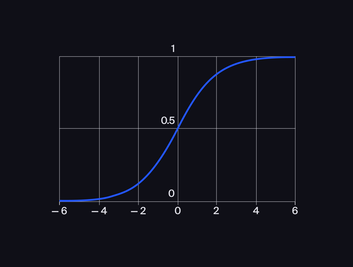
The latter diagram has the sigmoid function or activation function. It takes any real number as the input and returns a number in the range from 0 (no activation) to 1 (activation).

\sigma(z)=\frac{1}{1+e^{-z}}

This number in the range from 0 to 1 can be interpreted as a prediction of a neural network on whether the observation belongs to the positive class or the negative class.

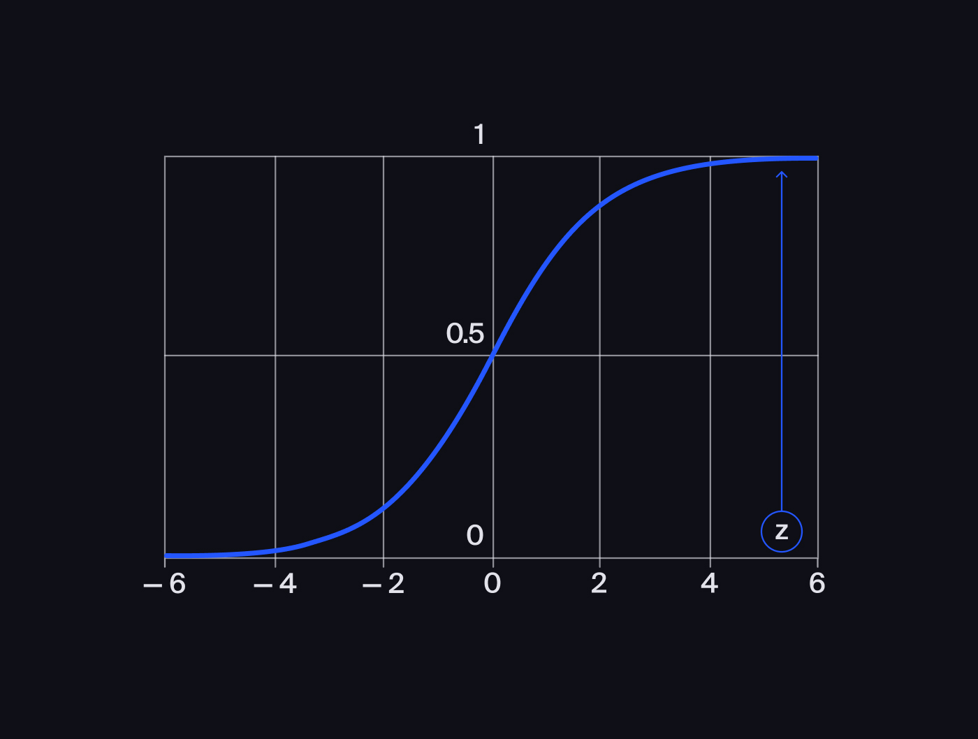
If the sum of the products of the inputs' values and the weights ( $z$ ) is very large, then at the sigmoid output, we'll get a number close to unity:

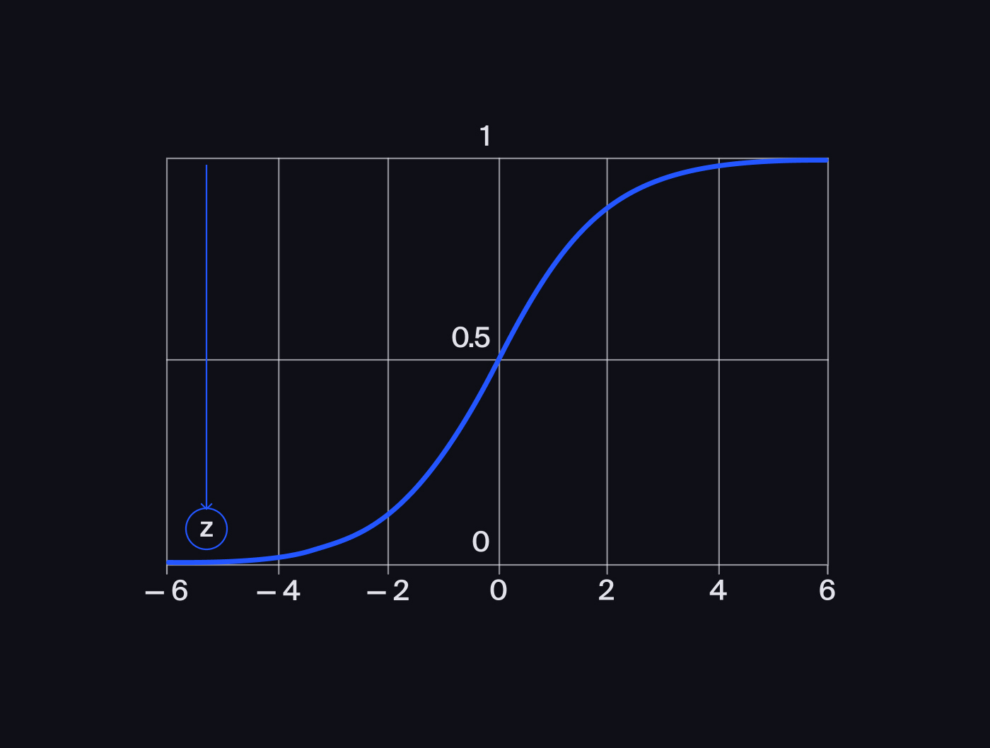
But if, on the contrary, the sum is a large negative number, then the function returns a number close to zero:

The loss function varies depending on the neural network type. The MSE is used in regression tasks, while Binary Cross-Entropy (BCE) is suitable for a binary classification. We can't use the accuracy metric because it doesn't have a product, making it impossible for SGD to work.

BCE is calculated as follows:

\text{BCE}=-\log{p}

In the formula, p is the correct answer probability. The base of the logarithm doesn't matter because the change of the base is the multiplication of the loss function by the constant, which doesn't change the minimum.

If the target = 1, then the correct answer probability is:

p=\sigma(z)

If the target = 0, then $p$ is:

p=(1-\sigma(z))

To better understand the BCE function, take a look at its graph:

If the correct answer probability $p$ is approximately equal to unity, then $-\log(p)$ is a positive number close to zero. Therefore, the error is small. If the correct answer probability $p≈0$ , then $-\log(p)$ is a large positive number. Therefore, the error is large.

Logistic Regression in Keras

To get a logistic regression, we only need to change the linear regression code in two places:

Apply the activation function to the fully connected layer:


1keras.layers.Dense(units=1, input_dim=features_train.shape[1],
2                  **activation='sigmoid'**)

Change the loss function from MSE to binary_crossentropy:


1model.compile(**loss='binary_crossentropy'**, optimizer='sgd')

Fully Connected Neural Networks

In fully connected neural networks every neuron in each layer is connected with each neuron of the previous layer.

Note that all the layers except for the input and output layers are called hidden layers

Every neuron except for the last one is followed by an activation function.

To get z, sum up all the products of the input values and the weights:

\begin{aligned} z_1 &= x_1 * w_{11} + x_2 * w_{12} \\ z_2 &= x_1 * w_{21} + x_2 * w_{22} \\ z_3 &= z_1 * w_{31} + z_2 * w_{32} \end{aligned}

We get:

z_3 = (x_1 * w_{11} + x_2 * w_{12}) * w_{31} + (w_{21} * x_1 + w_{22} * x_2) * w_{32}

Take $x_1$ and $x_2$ out of the brackets:

z_3 = x_1 * (w_{11} * w_{31} + w_{21} * w_{32}) + x_2 * (w_{12} * w_{31} + w_{22} * w_{32})

For convenience, we'll introduce new notation, $w_1^\prime$ and $w_2^\prime$ :

\begin{aligned} w_{1}^\prime &= w_{11} * w_{31} + w_{21} * w_{32} \\ w_{2}^\prime &= w_{12} * w_{31} + w_{22} * w_{32} \end{aligned}

We get:

z_3 = x_1 * w_1^\prime + x_2 * w_2^\prime

Here's the diagram of this formula:

A multilayer network is a single neuron network!

To fix this we reintroduce the sigmoid and see how the network changes:

The formula for this is:

\begin{aligned} z_1 &= \sigma (x_1 * w_{11} + x_2 * w_{12}) \\ z_2 &= \sigma (x_1 * w_{21} + x_2 * w_{22}) \\ z_3 &= z_1 * w_{31} + z_2 * w_{32} \end{aligned}

And we get:

z_3 = \sigma (x_1 * w_{11} + x_2 * w_{12}) * w_{31} + \sigma (w_{21} * x_1 + w_{22} * x_{2}) * w_{32}

Because of the sigmoids, we can't take $x_1 and $x_2$ out of the brackets. Meaning we aren't dealing with a single neuron now. The sigmoids allow for making the network more complex.

How Neural Networks are Trained

Similar to linear regression, multilayer networks are trained with gradient descent.

How does a neural network change when we add neurons and layers? To find out, solve a few tasks on the TensorFlow Playground website. This platform allows you to train small neural networks on model data with two features for classification tasks.

As the number of layers increase, the training gets less efficient. This is called a vanishing signal and is caused by the sigmoid, which converts large values into smaller ones over and over again.

To get rid of the problem, you can try another activation function, for example, ReLU (Rectified Linear Unit). Here's what it looks like:

And here's the ReLU formula:

\text{ReLU}=\max (0,x)

ReLU brings all negative values to 0 and leaves positive values without changes.

Fully Connected Neural Networks in Keras

Fully connected layers in Keras can be created by calling Dense(). To build a multilayer fully connected network, you need to add a fully connected layer several times.


1model = keras.models.Sequential()
2
3model.add(keras.layers.Dense(
4  units=10,
5  input_dim=features_train.shape[1],
6  activation='sigmoid')
7)
8
9model.add(keras.layers.Dense(units=1, activation='sigmoid'))
10
11model.compile(
12  loss='binary_crossentropy',
13  optimizer='sgd',
14  metrics=['acc']
15)
16
17model.fit(
18  features_train,
19  target_train,
20  epochs=10,
21  verbose=2,
22  validation_data=(features_valid, target_valid)
23)

Working with Images in Python

If the image is black and white, then each pixel stores a number from 0 (black) to 255 (white).

Let's open this image with the PIL (Python Imaging Library) library tools so we can work with it like with a NumPy array:


1import numpy as np
2from PIL import Image
3
4image = Image.open('image.png')
5image_array = np.array(image)
6print(image_array)


1[[255 255 255 255 237 217 239 255 255 255 255 255 255]
2 [255 255 190  75  29  29  30  81 198 255 255 255 255]
3 [255 147  30  29  29  29  29  29  31 160 255 255 255]
4 [185  29  29  29  29  29  29  29  29  31 198 255 255]
5 [ 61  29  29  29  29  29  29  29  29  29  74 255 255]
6 [108 121 121 121 121 121 121 121 121 121 102 219 255]
7 [250 255 255 255 255 255 255 255 255 255 238 107 168]
8 [255 238 153 150 152 244 201 152 150 178 253 103 144]
9 [248 243 121 108 114 225 184 130 112 154 235 103  62]
10 [197 255 227 168 231 149 230 196 179 251 183  29  29]
11 [105 255 255 219 195 191 184 195 235 255  91  29  29]
12 [ 30 187 255 234 218 218 218 218 243 174  29  29  29]
13 [ 29  38 180 255 255 255 255 255 169  35  29  29  29]
14 [ 29  29  29  82 153 174 150  76  29  29  29  29  29]
15 [ 29  29  29  29  29  29  29  29  29  29  29  29  29]]

We get a two-dimensional array.

Call the plt.imshow() (image show) to plot the image.


1plt.imshow(image_array)

You can plot the image in black and white by adding cmap='gray' argument. To add a color bar to the image, you need to call plt.colorbar().


1plt.imshow(image_array, cmap='gray')
2plt.colorbar()

Usually, neural networks learn better when they receive images in the range from 0 to 1 as input. To bring the scale [0, 255] to [0, 1], divide all the values of the two-dimensional array by 255.


1image_array = image_array / 255.

Color Images

Color images or RGB images consist of three channels: red, green, and blue. These images are three-dimensional arrays with cells containing integers in the range from 0 to 255.

Three-dimensional arrays in NumPy work just like two-dimentional ones.


1np.array([[0, 255],
2          [255, 0]])


1np.array([[[0, 255, 0], [128, 0, 255]],
2          [[12, 89, 0], [5,  89, 245]]])

In a three-dimensional array obtained from an image the first coordinate is the row ID, and the second one is the column ID. But here we also have a new third coordinate indicating the channel.

A three-dimensional array is just like a two-dimensional array from a black and white image. The difference being that each pixel of this array stores three numbers that represent the brightness of each of the three channels: red, green, and blue.

Multiclass Classification

This classification implies that the observations belong to one of several classes as opposed to one of two classes.

Suppose we have three classes. Here's the logistic regression represented as a neural network:

We get a fully connected network with the output layer containing not one, but three neurons. Each neuron is responsible for its own class. If the value at the $z_1$ output is a large positive number, then the network will set the observation to class "1."

How do we calculate the loss function? Remember the binary cross-entropy:

\text{BCE}=-\log{p}

If the target value is 1, then the correct answer probability is:

p=\sigma(z)

If the target value is 0, the $p$ -value is:

p=(1-\sigma(z))

We have three classes, but it won't affect the loss function calculation. And it will be called CE (cross-entropy):

\text{CE}=-\log{p}

In the formula, $p$ is the correct answer probability returned by the network.

Where do we get the probability from? Sigmoids are used to get it. What if we put a sigmoid after each neuron in the output layer?

\begin{aligned} p_1 \text{ (first class probability)} &= \sigma(z_1) \\ p_2 \text{ (second class probability)} &= \sigma(z_2) \\ p_3 \text{ (third class probability)} &= \sigma(z_3) \end{aligned}

All the probabilities are in the range from 0 to 1, but the sum of all three won't necessarily equal unity. If we assume that the observation belongs to only one class, we hope to get this:

p_1 + p_2 + p_3 = 1

The activation function that suits this case is called SoftMax. It takes several outputs of the networks and returns probabilities that are all equal to one.

\text{SoftMax}(z_i)=\frac{\exp(z_i)}{\sum_j \exp(z_i)}

Here's how we calculate the probabilities:

\begin{aligned} p_1 = \text{SoftMax}(z_1) &= \frac{e^{z_1}}{(e^{z_1} + e^{z_2} + e^{z_3})} \\ p_2 = \text{SoftMax}(z_2) &= \frac{e^{z_2}}{(e^{z_1} + e^{z_2} + e^{z_3})} \\ p_3 = \text{SoftMax}(z_3) &= \frac{e^{z_3}}{(e^{z_1} + e^{z_2} + e^{z_3})} \end{aligned}

Now $p_1$ varies in the range from 0 to 1.

Note that if $z_1$ is significantly greater than $z_2$ and $z_3$ , then in the first formula the numerator is approximately equal to the denominator, that is $p_1 \approx 1$ .

If $z_1$ is significantly less than $z_2$ or $z_3$ , then the numerator is much less than the denominator, that is $p_1 ≈0$ .

Now the probabilities are equal to one:

\begin{aligned} p_1 + p_2 + p_3 &= \text{SoftMax}(z_1) + SoftMax(z_2) + SoftMax(z_3) \\ &= \frac{e^{z_1}}{(e^{z_1} + e^{z_2} + e^{z_3})} + \frac{e^{z_2}}{(e^{z_1} + e^{z_2} + e^{z_3})} + \frac{e^{z_3}}{(e^{z_1} + e^{z_2} + e^{z_3})} \\ &= \frac{(e^{z_1} + e^{z_2} + e^{z_3})}{(e^{z_1} + e^{z_2} + e^{z_3})} \\ &= 1 \end{aligned}

Here's the diagram of our neural network with the SoftMax activation function:

Why does the SoftMax block in the diagram depend on all the outputs from the network? It's because we need all the outputs to find all probabilities.

If there are more than three classes, the number of the neurons in the output layer should be equal to the number of classes, and all outputs should be connected to SoftMax.

Probabilities from SoftMax at the training stage will go to cross-entropy, which will calculate the error. The loss function will be minimized using the gradient descent method. The only condition for the gradient descent to work is that the function has a derivative for all the parameters: weights and the bias of the neural network.

Let's see how the code changes. Here's the last layer initialization for binary classification:


1Dense(units=1, activation='sigmoid'))

And here's the initialization for multiclass classification:


1Dense(units=3, activation='softmax'))