Vectors and Vector Operations

Creating vectors

In mathematics, an ordered set of numerical data is a vector, or an arithmetic vector. In Python, operations with vectors are hundreds of times faster than operations with lists.

To work with vectors use the NumPy library.


1import numpy as np
2
3numbers1 = [2, 3] # Python list
4vector1 = np.array(numbers1) # NumPy array
5print(vector1)

Vectors can be created without a temporary variable:


1import numpy as np
2vector2 = np.array([6, 2])
3print(vector2)

Vectors can be converted into lists:


1numbers2 = list(vector2) # List from vector
2print(numbers2)

The column of the DataFrame structure in pandas is converted into a NumPy vector using the values attribute:


1import pandas as pd
2
3data = pd.DataFrame([1, 7, 3])
4print(data[0].values)

Use the len() function to determine the vector size (number of its elements):


1print(len(vector2))

Vector presentation

The vector is represented by a point or an arrow that connects the origin and the point with coordinates (x, y). We use arrows when we want to indicate the movements.

Vector elements are also called coordinates.


1import numpy as np
2import matplotlib.pyplot as plt
3
4vector1 = np.array([2, 3])
5vector2 = np.array([6, 2])
6
7plt.figure(figsize=(7, 7))
8plt.axis([0, 7, 0, 7])
9# 'ro' argument sets graph style
10# 'r' - red
11# 'o' - circle
12plt.plot([vector1[0], vector2[0]], [vector1[1], vector2[1]], 'ro')
13plt.grid(True)
14plt.show()

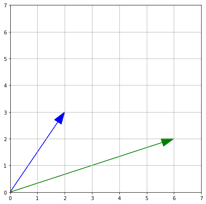
Let's use arrows to draw the same vectors. Instead of plt.plot(), call plt.arrow().


1import numpy as np
2import matplotlib.pyplot as plt
3
4vector1 = np.array([2, 3])
5vector2 = np.array([6, 2])
6
7plt.figure(figsize=(7, 7))
8plt.axis([0, 7, 0, 7])
9plt.arrow(0, 0, vector1[0], vector1[1], head_width=0.3,
10          length_includes_head="True", color='b')
11plt.arrow(0, 0, vector2[0], vector2[1], head_width=0.3,
12          length_includes_head="True", color='g')
13plt.plot(0, 0, 'ro')
14plt.grid(True)
15plt.show()

Addition and subtraction of vectors

Vectors of the same size have equal length. The result of their addition is the vector with each coordinate being equal to the sum of the coordinates of the summand vectors.

When adding or subtracting vectors, the operation is performed for each element of the vectors:

Vector	Coordinates
$\bar{x}$	$(x_1,x_2,\dots,x_n)$
$\bar{y}$	$(y_1,y_2,\dots,y_n)$
$\bar{x}+\bar{y}$	$(x_1+y_1,x_2+y_2,\dots,x_n+y_n)$
$\bar{x}-\bar{y}$	$(x_1-y_1,x_2-y_2,\dots,x_n-y_n)$


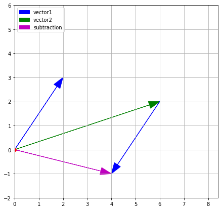
1import numpy as np
2
3vector1 = np.array([2, 3])
4vector2 = np.array([6, 2])
5sum_of_vectors = vector1 + vector2
6subtraction_of_vectors = vector2 - vector1

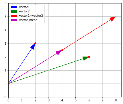
If we plot a vector that is equal to the green vector1 in terms of length and direction from the end of the blue vector2, we will get the red vector (sum_of_vectors).

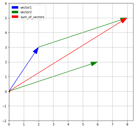
If each vector is a movement in a certain direction, then the sum of two added vectors is the movement along the first vector followed with the movement along the second one.

The difference of two vectors is a step — for example along vector2 — followed by a step along the direction opposite to vector1.

Multiplication of a vector by a scalar

Besides addition and subtraction, vectors can be also multiplied by scalars. Each coordinate of the vector is multiplied by the same number:

Vector	Coordinates
$\bar{x}$	$(x_1,x_2,\dots,x_n)$
$k\bar{x}$	$(kx_1,kx_2,\dots,kx_n)$

If the number is negative, all coordinates also change their signs.


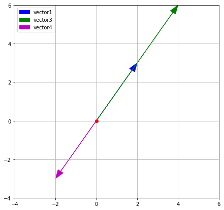
1import numpy as np
2
3vector1 = np.array([2, 3])
4vector3 = 2 * vector1
5vector4 = -1 * vector1

When multiplied by a positive number, vectors on the plane maintain direction, but the arrows change length. When multiplied by a negative number, vectors flip to the opposite direction.

Mean value of vectors

For the set of vectors $a_1,a_2,\dots,a_n$ (where $n$ is the total number of vectors), the mean value of vectors is the sum of all vectors multiplied by $\frac{1}{n}$ . This results in a new vector $a$ .

a=\frac{1}{n}(a_1+a_2+\dots+a_n)

If the set consists of only one vector ( $n=1$ ), it will be equal to the mean: $a=a_1$ . The mean value of two vectors is $a=0.5(a_1+a_2)$ . The mean value for a pair of two-dimensional vectors is the middle of the segment connecting $a_1$ and $a_2$ .


1import numpy as np
2
3vector1 = np.array([2, 3])
4vector2 = np.array([6, 2])
5vector_mean = .5*(vector1+vector2)
6print(vector_mean)

The first coordinate of the new vector is the mean value of the first coordinates of vector1 and vector2, and the second coordinate is the mean value of the second coordinates of vector1 and vector2.

That's how we draw these vectors on the plane: plot the vector1+vector2 vector and then multiply it by 0.5.

Vectorized Functions

If we use the np.array() function after multiplying and dividing two arrays of the same size, we will obtain a new vector that will also have the same size:


1import numpy as np
2
3array1 = np.array([2, -4, 6, -8])
4array2 = np.array([1, 2, 3, 4])
5array_mult = array1 * array2
6array_div = array1 / array2
7print("Product of two arrays: ", array_mult)
8print("Quotient of two arrays: ", array_div)

If arithmetic operations are performed on an array and a single number, then the action is applied to each element of the array. And an array of the same size is formed.


1import numpy as np
2
3array2 = np.array([1, 2, 3, 4])
4array2_plus_10 = array2 + 10
5array2_minus_10 = array2 - 10
6array2_div_10 = array2 / 10
7print("Sum: ", array2_plus_10)
8print("Difference: ", array2_minus_10)
9print("Quotient: ", array2_div_10)

The same element-by-element principle works on arrays when we deal with standard mathematical functions like exponentiation or logarithms.

Let's raise an array to the second power:


1import numpy as np
2
3numbers_from_0 =  np.array([0, 1, 2, 3, 4])
4squares = numbers_from_0**2
5print(squares)

All of that can be done with lists using loops as well, but operations with vectors in NumPy are much faster.

Here's the formula of the min_max_scale() function:

f(x)=\frac{x-\min}{\max-\min}

To apply this function to all elements of the values array, call the max() and min() methods. They will find its maximum and minimum values. As a result, we get an array of the same length, but with converted elements:


1import numpy as np
2def min_max_scale(values):
3    return (values - min(values)) / (max(values) - min(values))
4
5print(min_max_scale(our_values))

To apply this function to all elements of the values array, call the max() and min() methods. As a result, we get an array of the same length, but with converted elements:

f(x)=\frac{1}{1+\exp{(-x)}}

exp() is the exponent function, it raises $e$ which approximately equals 2.718281828.

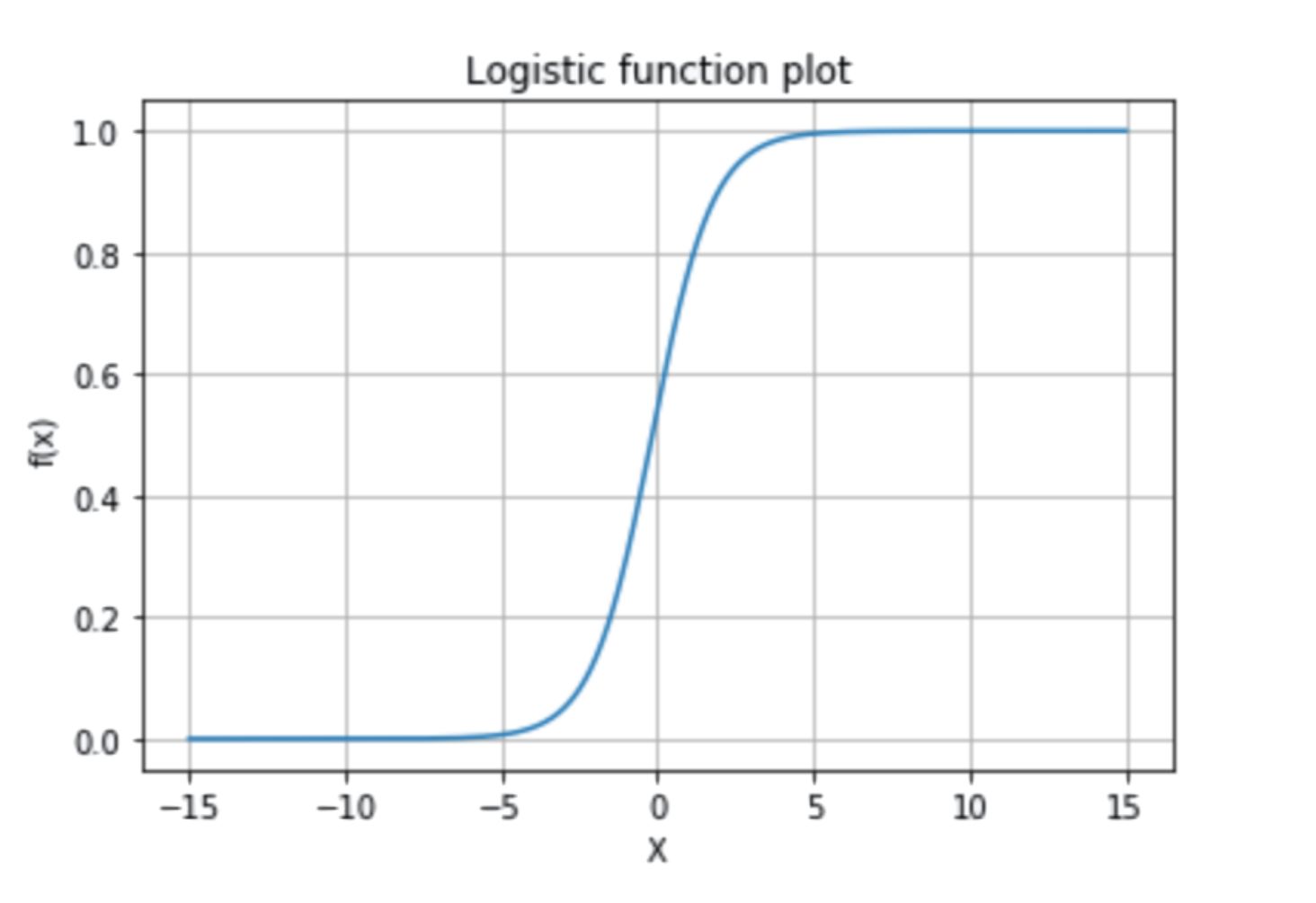
Perform logistic transformation:


1import numpy as np
2
3def logistic_transform(values):
4    return 1 / (1 + np.exp(- values))
5
6print(logistic_transform(our_values))

Vectorization of metrics

Store a set of actual values to the target variable, and predicted values to the predictions variable. Both sets are np.array type.

Use standard numpy functions to calculate the evaluation metrics:

sum() (to find the sum of the elements in an array)
mean() (to calculate the mean value)

Call them as follows: <array name>.sum() and <array name>.mean().

Here's the formula to calculate the mean square error (MSE)

\text{MSE}=\frac{1}{n}\displaystyle\sum^n_{i=1}(\text{target}_i-\text{predictions}_i)^2

where $n$ is the length of each array and $\sum$ is the summation over all observations of the sample ( $i$ varies from $1$ to $n$ ). The ordinal elements of the vectors target and predictions are denoted by $\text{target}_i$ and $\text{predictions}_i$ .


1def mse1(target, predictions):
2    n = target.size
3    return((target - predictions)**2).sum()/n

Write the MSE formula using mean()


1def mse2(target, predictions):
2    return((target - predictions)**2).mean()

Write the function to calculate MAE using mean()

\text{MAE}=\frac{1}{n}\displaystyle\sum^n_{i=1}|\text{target}_i-\text{predictions}_i|


1import numpy as np
2
3def mae(target, predictions):
4    return np.abs((target - predictions)).mean()
5
6print(mae(target, predictions))

Vectorized functions can be used to calculate RMSE.

\text{RMSE}=\sqrt{\text{MSE}}=\sqrt{\frac{1}{n}\displaystyle\sum^n_{i=1}(\text{target}_i-\text{predictions}_i)^2}


1import numpy as np
2
3def rmse(target, predictions):
4    return (((target-predictions)**2).mean())**0.5
5
6print(rmse(target, predictions))